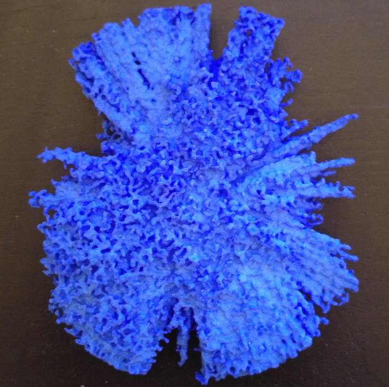
A 3D print of the largest connected region in the 5% mesh.
A mesher takes scalar field slices (such as described in my previous blog post) and a scalar value v and outputs an isosurface mesh such that the surface has value v everywhere, typically using the Marching Cubes algorithm. In this case, these are isosurfaces of constant density.
I used the SliceCubes() function in the Python version of the VTK library to convert the slices to meshes using the VTK implementation of the Marching Cubes algorithm.
I computed a mesh for each density value from 0.99 (99%) to .05 (5%) in 0.01 (1 percent) increments, or 95 meshes in all. The lowest density value of 0.05 (5%) corresponds to 3.33 x 10**(-4) stars per 3x3x3 bin.
I kept a list of the stars contained in each connected region (for future data mining) and output each connected region containing 5 or more stars as a separate mesh.
A typical density mesh may contain hundreds of connected regions. For all the density levels combined, there were 33239 connected regions.
The largest connected region in the 5% density mesh contains 297498 stars, which is 97% of all the stars in the 5% density mesh and 88% of all the stars in the cylinder being mapped. I made a 3D print of this region (displayed in the picture at the top of this blog post).
All of the regions in the galaxy map are inside the 5% density mesh and hence essentially all are inside the 3D print shown above.
But how to choose which of the more than 33 thousand regions to include in the map?
The regions are nested in the sense that all the regions with a density value v1 are contained in regions with density value v2 if v1 > v2.

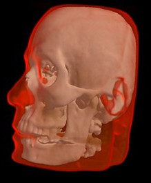
A medical render with two translucent density levels.
Typically, for example, in MRI scans, this density difference (for example between bone and other tissue) is used to render a meaningful display by selecting all the regions from a small range of density values (perhaps 2 to 4) and displaying them using nested translucent meshes.
Indeed I used a similar technique to display TGAS regions from Gaia DR1.
But now we reach the fundamental problem with mapping star distribution using density isosurfaces in Gaia DR2. With medical applications such as MRI scans or in regions of low extinction such as the solar neighbourhood, the density values are well defined. This is not the case for Gaia DR2. Because of dust reddening, instrument magnitude limits and other selection effects, two regions that in reality may have similar star density may have very different density values in Gaia DR2.
How do we map star concentrations using density isosurfaces when the real density values are uncertain?
In my next blog post I will describe how I solved this problem and present what I believe is a new technique for mapping density isosurface regions in the presence of density uncertainty.
