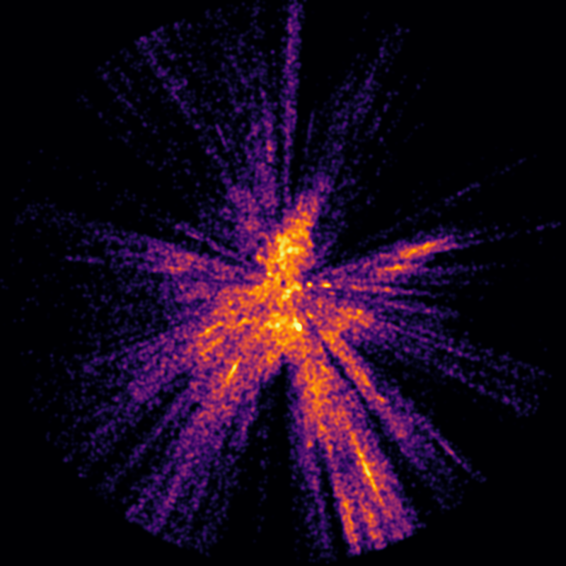
An example hot star density slice (in this case near the galactic plane).
In order to apply the isosurface mapping technique, we must convert a point cloud, such as the set of about 340 thousand hot O, B and early A class stars I described in my last blog post, into a scalar field, a real valued function defined in principle for every point in euclidean space (or at least in a defined grid). This scalar field is in some way a measure of star density. We can then extract isosurfaces of constant density from this scalar field, much as contour lines are lines of constant elevation on a topographic map of mountainous terrain on Earth.
In order to make the necessary calculations manageable on my 16 Gb workstation, I placed the density values into 3x3x3 parsec bins.
I represented the cylinder mentioned in my last blog post (with a radius of 3000 parsecs and height 600 parsecs above and below the galactic plane) as a subset of a 6000 x 6000 x 1200 pc box and reduced this into 2000 x 2000 x 400 bins (with dimensions 3x3x3 pc) in a numpy array.
I then counted the number of stars in each bin. This created a scalar field of sorts, but a very discontinuous one.
I borrowed the gaussian smoothing technique mentioned in H. Bouy and J. Alves 2015, "Cosmography of OB stars in the Solar neighbourhood". For the map I chose a a gaussian sigma of 15 parsecs. The choice of a gaussian sigma is as much an aesthetic choice as it is a scientific one. The higher the sigma, the less detailed the map. A low sigma results in a chaotic map. A high sigma results in a smooth map with limited detail. I experimented with several values before settling on 15 parsecs.
Fortunately, the Python library scipy.ndimage.filters has an appropriate gaussian_filter function that could be applied directly to the numpy array.
In addition, for ease in future processing, I wanted to ensure that the values of the density function ran between 0 and 1.
There are numerous ways to normalize the density values in this way (for example dividing by the maximum value). The option I chose is to use this variation of the sigmoidal logistic function:
f(x) = 2/(1+exp(-kx)) - 1
which ranges between 0 and 1 in an S-shaped curve as x ranges between 0 and infinity.
This sigmoidal value stretching / normalization is often used in image processing to continuously compress data with very high and low values into a smoother middle range. As with the gaussian sigma value, the logistic k value is partly an aesthetic choice. A low k value pushes the function towards 0. A high value pushes the function towards 1. After experimenting with various values for k, I selected 300. This seemed to more evenly spread the possible density values between 0 and 1.
The scipy.special library has an expit function that can be applied to numpy arrays.
I then sliced the cylinder values in the numpy box from top to bottom in 3 pc slices and output the results as coloured 8 bit images (for debugging the sigma and k values) and as 16 bit pgm values (needed for isosurface generation). One of the coloured slice images is at the top of this blog post.
Once the slices were done, I could move on to the next stage: meshing.
