Last week I released a map of the Milky Way within 3000 parsecs (10 thousand light years) of the Sun made using data from Gaia DR2 and several other sources as described on my previous blog post.
You can see a face-on web version here or view the full 3D meshes in the latest version of Gaia Sky.
This week I'm starting a series of blog posts to explain in detail how I created the map. I hope that these posts will be useful for others who might want to try the density isosurface technique to create their own maps. At the end of this series I'll link to relevant resources, including the map meshes, SVG and Blender files, and Python source code.
The Gaia DR2 archive provides parallaxes for more than a billion stars, but I used only a tiny fraction of these to create the actual map. First, I selected only the stars with the most accurate parallaxes in the Gaia DR2 data set, the 72 million stars with error/parallax < 0.1.
There is a field in the Gaia DR2 database that is the reciprocal of this value, parallax_over_error. So in practice I was selecting the stars with parallax_over_error > 10.
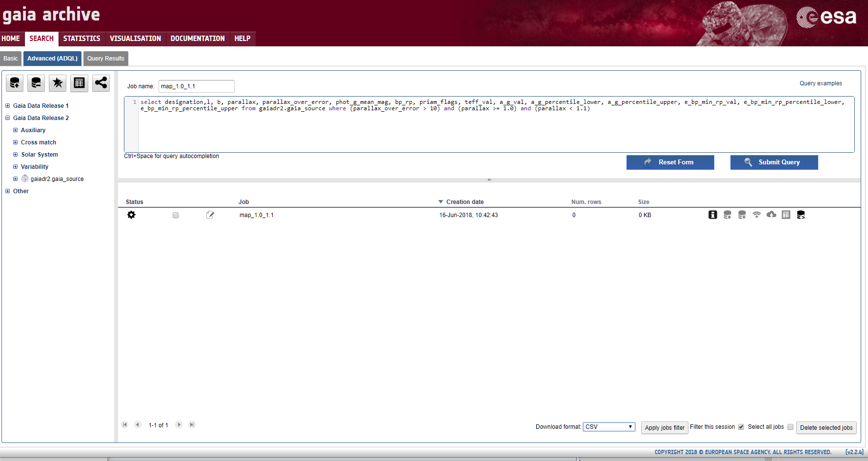
The main difficulty with extracting this data set from the Gaia archive was the time. For the main archive, there is a maximum query limit of 30 minutes and at the time I was using the archive, selecting the data was slow. I ended up splitting the data selection into 28 queries based on the parallax value. A sample query is shown in the image at the top of this blog post. It took most of a day to get all the data. I do wonder if the Gaia database administrators might consider allowing faster downloads for commonly used data subsets.
After acquiring the data, I applied a few quality cuts and selected only about 400 thousand very hot O, B and early A class stars using a colour index filter with colour index < 0 and added an absolute magnitude cut (absolute magnitude < 7) to filter out dim but hot non-main sequence stars like white dwarfs. (Actually the hot stars I was mapping all have an absolute magnitude much brighter than 7. I chose that number to compensate for some dust extinction as well.)
The Gaia DR2 database includes a raw colour index value bp_rp, and a second colour excess value, e_bp_min_rp_val, that attempts to correct for dust reddening.
So we can define colour index = bp_rp - e_bp_min_rp_val.
These values are a relatively simple estimate of what Gaia will ultimately be capable of - more accurate colour values will be provided in Gaia DR3.
Filtering to these hot, young stars was an essential part of making the map possible. Cooler, older stars tend to drift randomly from their sites of formation. I tried a number of experiments to map cooler stars without a great deal of success - they were either present in a large number of random clumps or, at lower density levels, just a few large areas.
In contrast, hot young stars are largely gathered in dense associations, mostly near the galactic plane. Their distribution, especially those regions containing the ultra hot O-B3 class ionizing stars, form a distinct (and hence mappable) pattern.
After the colour selection, I further filtered to all stars within a cylinder with a radius of 3000 parsecs and a height of 600 parsecs above and below the galactic plane.
Why the 3 kpc limit? The main reason is that stars with very accurate parallaxes (err/plx < 0.1) start to fade out beyond 3.6 kpc. I definitely wanted to include the Carina nebula, which is more than 2 kpc away. The further I extended the map, the less accurate the star positions became, and also, more pragmatically: most of the structures (eg. OB associations or HII regions) that astronomers have named turn out to lie within 3 kpc. So a 3 kpc limit allowed the most accurate map with names for most of the major regions.
The 600 parsec height limit was a bit arbitrary and was mostly to reduce memory consumption. This did result in some truncation for a few very low density regions. An interesting alternative map might ignore the thin disk and look for density structures in the thick disk and halo.
This distance cut gave me a final data set of about 340 thousand stars, ready for the next stage of density isosurface generation - slicing.

