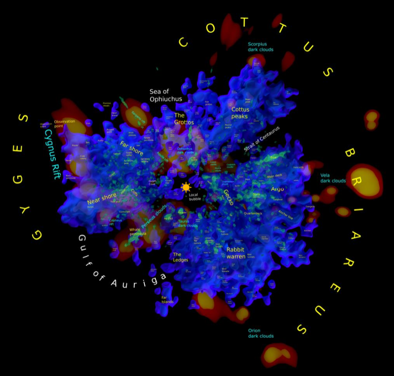
I have used the TGAS (Tycho-Gaia Astrometric Solution) data released as part of Gaia DR1 to create a topographic map of the solar neighbourhood within a distance of 800 parsecs.
Caveats
Links to various ways to see the map are below. First, some caveats:
- The TGAS data is known to be incomplete. A more complete and accurate data set extending far beyond the solar neighbourhood into the spiral arms and the galactic nucleus is scheduled to be released in April 2018. For now TGAS is the best data we have for mapping the Milky Way.
- This is a topographic map showing isosurfaces of constant star density and is analogous to a hiking map showing isolines of constant elevation. If you want a visualization showing, for example, what it would be like to fly through the Hyades cluster, this is not it. For direct visualizations of the star data, you might want to look at Gaia Sky.
- When generating the map, I created names for several hundred isosurface peaks, analogous to mountain peaks or ranges on a hiking map. Although in many cases these names have been inspired by Greek mythology or other traditional star lore, the names are in no way official and were created largely because it is easier for me to remember them and their locations on the map than isosurface region identifiers like TR1 40-54. Only the International Astronomical Union (IAU) can give official names to celestial objects.
The density functions
The isosurfaces on this map are each defined by a density value. The density value is determined by a star density function. There are two density functions used for this map. The first is computed from 20 thousand hot stars (colour index <= 0). The second is computed from 400 thousand bright stars (absolute magnitude <= 3).
In both cases the density functions are computed by filtering for low error stars in the TGAS data set (err/plx < 0.2), counting the number of stars (hot or bright) in each bin of a 2x2x2 grid and then applying a gaussian smoothing function to define a scalar field for each cubic parsec. For the hot star isosurfaces I used a fairly large gaussian sigma of 15 parsecs. For the bright star isosurfaces I used a smaller gaussian sigma of 5 parsecs, resulting in a larger number of smaller isosurfaces compared to the larger sigma.
The net effect is that the hot star isosurfaces identify large regions in space and the bright star isosurfaces define smaller clumps of bright stars.
The density functions range between 0 and a maximum value. I have used an exponential spread function to normalize this range to between 0 and 1. A specific isosurface can be defined by selecting a value between 0 and 1 (or more conveniently between 0 and 100). The 0% isosurface contains all the density values >= 0 and so in both cases is a solid sphere. As the density value rises, the number of disconnected isosurface regions starts to multiply and their size is reduced. Eventually as the density value reaches 100%, there are only a few very dense star clumps remaining.
Panurania and the stellar continents
As I mentioned in some blog posts last year, the majority of hot stars can be found in a single isosurface up to and including a density value of about 30%. I have called this stellar supercontinent Panurania (Urania being the Muse of Astronomy and a great granddaughter of Ouranos/Uranus, the god of the heavens). It has many branches and empty spaces and resembles a gigantic Red Ridge sponge.
After 30%, Panurania breaks up into three stellar continents. It seems logical to name these after children of Ouranos and Gaia. The most famous of their children, the Titans, have been widely used for names of moons and asteroids. However, besides the Titans, their children also include the Cyclops and the hundred-armed Hecatoncheires, whose names seem much less widely used.
Given that the stellar continents have many branches, I named them after the hundred-armed Hecatoncheires: Briareus, Gyges and Cottus.
Regions
The isosurfaces consist of hundreds (or for some density values thousands) of disconnected regions. I have given each region an identifier using the recommended IAU identifier system: a three character acronym followed by a region identifier. The set of "hot" isosurfaces are called TR1 (TGAS Regions 1) and the set of "bright" isosurfaces are called TR2.
The identifiers are made up of a isosurface density followed by a region number. For example, the Gyges stellar continent is TR1 40-15. This means that each isosurface has a formal identifier (TR1 40-15) as well as a more fanciful name (Gyges).
Some links
There is a lot to say about the map, but only a tiny amount will fit in a single blog post. I want to get on to providing some links.
It is much more difficult to visualize isosurfaces than isolines on a more familiar contour elevation map, because these density isosurfaces are three-dimensional and have complex shapes. When we look at an elevation map, isolines representing higher elevations can be found within isolines representing lower elevations. The same is true for isosurfaces. However, because isosurfaces are 3D, we must visualize surfaces appearing inside other surfaces, much like very complex Russian dolls.
So I have represented the map using many different images, all of which reveal an aspect of the map.
One way to do this is through animations. For example, this video shows a sequence of hot star isosurfaces fading or melting into each other from 20% to 95%. As the animation goes on, denser pockets of hot stars are revealed inside less dense regions:
(I recommend full screen and perhaps loop mode for all the animations I link to as there is a lot to see.)
Unfortunately this animation does not given you an idea of the complex 3D shapes of the isosurfaces. Below is a rotating view of the 40% hot star isosurface. I have simplified it by filtering the regions so that the visible regions contain 5 or more hot stars (the larger regions contain thousands of hot stars):
Even this view does not given you a clear view of the main stellar continents, so I have uploaded the Briareus, Gyges and Cottus isosurfaces to Sketchfab. You can click on each and view them in 3D here:
https://sketchfab.com/kevinjardine/collections/tgas
In the Sketchfab isosurfaces you can see that:
- Gyges has a complex structure, the Gyges reef, that extends below the galactic plane and appears below the local bubble. As I will show in another blog post, the OB association Lac OB1 is part of the Gyges reef
- Briareus has a saddle structure with parts that rise well above the galactic plane at either end.
- Cottus divides into two parts: the peaks and the grottoes. The peaks rise above the galactic plane and the grottoes descend well below it.
Of course, it is still useful to have a two-dimensional map, so I have provided a pannable and zoomable one here with quite a few viewing options:
http://galaxymap.org/gaia/tgas/topo/
I'll have a lot more to say about this 2D map in my next blog post, but for now you can click on the Help link at the bottom of the settings area at the upper right to read more about it.
Finally, I have uploaded the Python code I used to create the map and its various visualizations to GitHub here: