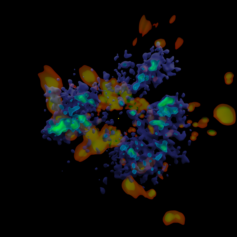
(Note: in all of these images, 0° galactic longitude is at the top, the Sun is at the centre, and the radius of the data is about 800 parsecs.)
Visualising isosurfaces is hard. They fit inside each other like very complex Russian dolls but no technique for showing several isosurfaces at once works perfectly.
A common technique is to make one isosurface partially transparent so you can see one inside the other, as is done in the image at the top of this article (which also includes the local dust clouds in orange and a yellow dot representing the location of the Sun). However, this only works for two or three surfaces and is difficult for the larger less-dense TGAS isosurfaces because of the complex sponge-like structure of the solar neighbourhood.
(The dust clouds in the above image are derived from data presented in this paper:
Lallement, R., Vergely, J. L., Valette, B., Puspitarini, L., Eyer, L., & Casagrande, L. (2014). 3D maps of the local ISM from inversion of individual color excess measurements. Astronomy & Astrophysics, 561, A91.)
Perhaps the simplest isosurface visualisation technique is an animation in which the larger isosurfaces evaporate to reveal the ones inside.
The following Youtube video was created using the hot star density isosurfaces I described in a previous blog post:
(The best view is 4K full screen.)
The lower density surfaces clearly reveal a crater-like structure in the third quadrant. This is caused by missing TGAS data in this quadrant and is not a real structure.
The animation is interesting, however a traditional map requires a still image or at least something that can be labelled.
Another option is to overlay several isosurfaces on top of each other. This obscures the three dimensional structure but at least shows how one surface fits inside the other.
For example, this image shows the isosurfaces for which the star density is greater than or equal to d%, where d is 5, 55, 80 and 90:
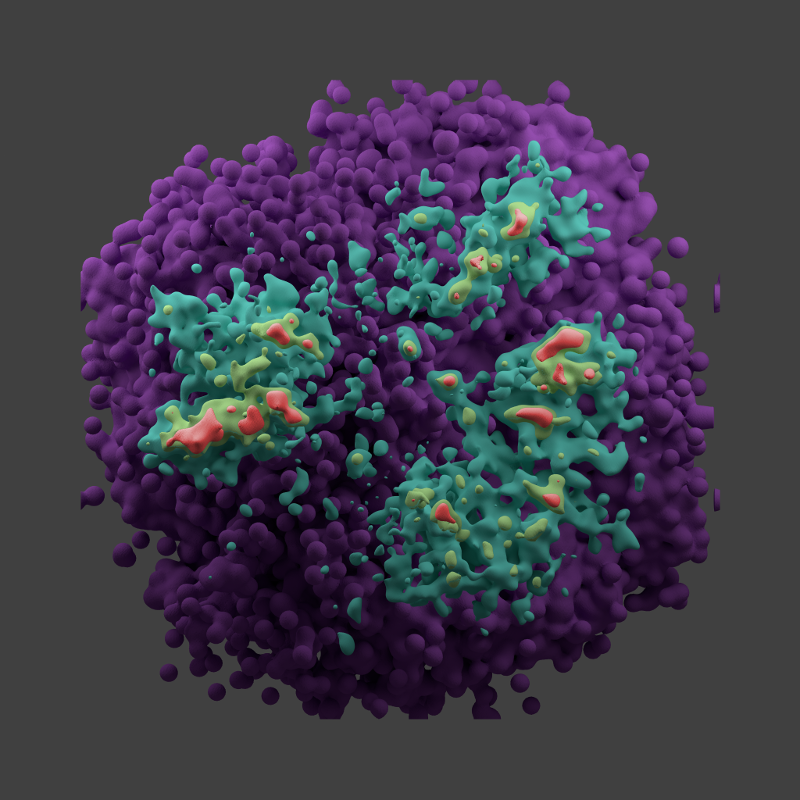
The highest 80% and 90% concentrations in this image and the one at the top of this post represent dense hot star concentrations, including OB associations.
You can see the three stellar "continents" of the solar neighbourhood in this image and the one created using three of these isosurfaces at the top of this blog post.
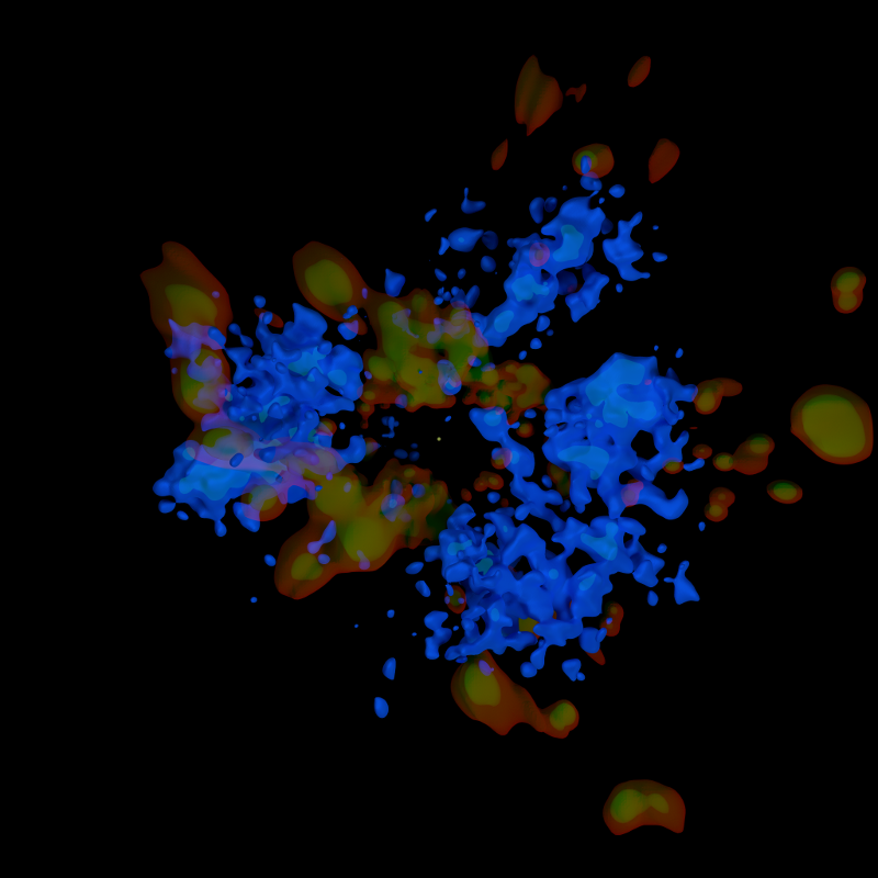
Here's another experiment, this time combining dust and the 60% and 85% isosurfaces:
A successful 3D map of the solar neighbourhood will likely require a combination of these techniques as viewed from several directions.
I hope in my next blog post to present the first draft of a real map of the solar neighbourhood with star clusters, dust clouds, hot star concentrations and labels. Given the limitations of the TGAS data, this first draft will inevitably be incomplete, but it will prepare the way for a more complete map when Gaia DR2 is released about a year from now.
The map will take a while to put together, so look for it early in the new year!