It is important to keep in mind that I'll really be using the temperature density function T(x,y,z) I mentioned in my last blog post to map the TGAS data, which is not quite the same thing as the stars in the solar neighbourhood.
TGAS looks a little like a donut with a 600 pc radius, a hole around the Sun, and a few large bites taken out of it. It has missing data. I'll discuss this missing data in more detail in a future post. For now, I'll take TGAS as it is.
We can construct a preliminary version of T(x,y,z) quite simply. For any point (x,y,z), round off the values to the integer point (i,j,k). Select all the TGAS stars in the one parsec cube centred on (i,j,k) with err/parallax < 0.2 and the colour index Ci < c where c is some value that appropriately selects hot stars. In my experiments below, I'll look at c = 0.0 and c = 0.1.
Then convert the Ci value for each star to temperature (I did that by interpolating Eric Mamajek's very useful table here). Add up all the temperatures for the stars in the cube. That is T(x,y,z). If there are no stars in the cube, set T(x,y,z) to zero.
This is a temperature density function of sorts but for our purposes it is not a very useful one. For mapping and presentation purposes we need a relatively smooth function that ranges between 0 and 1. What I have defined so far is a very discontinuous and spiky function. Fortunately there are some very common techniques that we can use to tame our function.
The first step is to de-spike the function. In astronomy, a common practice is to apply a de-spiking function to data to reduce it to a more manageable range. De-spiking functions commonly used are sqrt, ln or arcsinh. In my experiments with the TGAS data, I found a fourth root sqrt(sqrt(x)) works very well.
The second step is to smooth the function out over 3-dimensional space. A convenient way to do this is to apply a gaussian normal function. This is in effect a weighted average where the weight gets smaller the farther you are from the point. 2d gaussian smoothing is commonly used to reduce unwanted detail in photographs. 3D gaussian smoothing is similar except that it takes place in all three dimensions. The amount of smoothing is defined by the standard deviation σ (sigma). In the experiments below I look at σ values of 10 and 15 parsecs.
The final step is to clamp the values of the function between 0 and 1. One common clamp function is to just test to see if a value is > 1 and if it is, set it to 1. However, this introduces an ugly discontinuity into our function and we want something smoother. Another option is to find the largest value in our data set and divide all the other values by it. Although this does clamp the function in a continuous way, in many data sets, even after de-spiking, the maximum value can be large and this might create a function with a poor spread in values where only a few values are close to 1 and most other values are close to 0.
At this point I'd like to introduce one of my favourite tools for image processing, the sigmoid function. There are several variations of this, but the one I will use is:
f(x) = 2/(1+exp(-s*x)) - 1
where s is a constant called a spread.
This function uses the constant s to spread the values over a reasonable range and then the function guarantees that the values are smoothly clamped between 0 and 1.
De-spiking, smoothing and clamping are common image processing techniques that work just as well for 3D data sets. In this case, the range of possible temperature density functions is determined by the constants c, σ and s. Getting these constants right is important. Selecting the wrong c might exclude important hot stars or alternatively contaminate the data by introducing cooler stars that have drifted far from their origins. Selecting the wrong σ might remove important details from the data or alternatively fragment the data into too many small regions. Selecting the wrong s spread value might squeeze most of the data into too small a range.
It turns out that it was not that difficult to select reasonable spread values. The other values were more difficult so I tried some experiments with c = 0.0 and 0.1 and σ = 10 and 15.
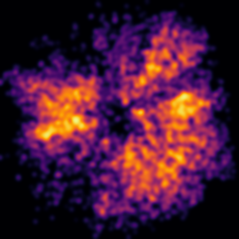
The results for the galactic plane are below (0° galactic longitude is at the top of the images):
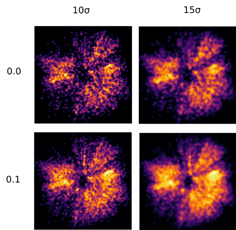
After looking at the various options (including animating full versions of the 3D dataset for all four parameter options) , I chose c = 0.0 and σ = 15. A larger version for the galactic plane using those values is at the top of this blog post.
You can journey through the full TGAS cube using this temperature density function in the animation here:
(best at 4K full screen or at least full screen).
There is a lot to see in this animation but a commentary will have to wait for a future blog post.