Suppose that you wanted to make a map of Europe and all you had was a satellite image taken at night. You might start with something like the image below.
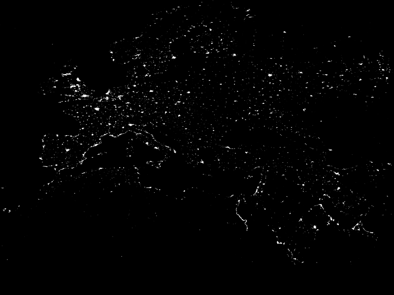
If you did a careful analysis of the distribution of the lights, you could extract quite a bit of information from this image, including the location of major cities and most of the coast line.
We have a similar situation with the TGAS data set. The distribution of the stars, especially the hotter stars, is by no means random. Using some mathematical tools, we can extract quite a bit of information about the solar neighbourhood out to about 800 parsecs (beyond this distance, the limited accuracy of the parallax measurements for even the brightest stars makes them impossible to place on a map).
One key tool is temperature density. The Tycho-2 catalog provides B and V magnitudes for almost all the stars. The difference B-V is called the colour index and it can be used to estimate the temperature of a star.
We are more likely to find structures to map using the hotter stars because these tend to be younger and younger stars are located close to the star formation regions within which they were born. (We can think of a star formation region as analogous to a city in a map of Earth.) Older, cooler stars often drift in random directions from their origin over time and so are less useful for mapping purposes.
Astronomers usually use the hottest O and B class stars to map star formation regions. These correspond to B - V < 0. However, I've been a bit more generous in my analysis because stars embedded in dust clouds can be reddened, increasing their colour index. So I've selected all the Tycho-2 stars with B-V < 0.1 to include some of the reddened B-class stars. In some cases this pulls in some hotter A-class stars but that should make little difference for the analysis.
I've interpolated Eric Mamajek's very useful table to convert colour index to effective temperature.
As usual, I am starting with the approximately 1 million stars in the TGAS data set with err/parallax < 0.2 for the reasons explained in my previous blog post on TGAS limitations.
In order to find structures, you have to have a way to aggregate individual star data. I've done this in two steps:
- Bin the data
- Smooth the data
In my first experiment, I calculated the x, y and z values in parsecs relative to the Sun. I defined my bins as all the stars with the same integer x and y values. For this first experiment, I ignored the z value, so this adds together all the stars with the same x and y parsec values above and below the galactic plane regardless of their z-height. I then added together the temperatures for all the stars in each bin with B-V < 0.1.
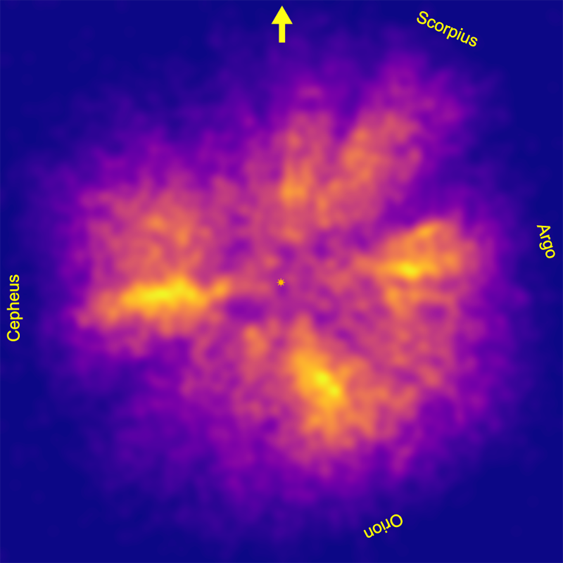
To smooth the data, I started by taking the square roots of the temperature sums to reduce the spikiness of regions with a lot of hot stars. I then used gaussian smoothing with a sigma (standard deviation) of 15 parsecs. The result of my first experiment is below. I have added the position of the sun at the centre, an arrow pointing in the direction of the galactic nucleus, and names for each of the four identified hot star concentrations. The full image (right to the edge of the rectangle) is 800x800 pc. You can see that the hot star density drops well before 800 pc.
It is much easier to visualise these density distributions as height maps, so I created and animated one in the 3D graphics application Blender. You can see the result on Youtube:
(I suggest going to full screen and right-clicking on the video to set the loop option as the animation is fairly fast.)
There are some surprising structures visible in these images, especially in the hot star concentration that I labelled Cepheus. I'll discuss some of them in my next blog post.